Getting started
The talon package, at its core, provides a way to transform a tractogram
into a linear operator, or more precisely a matrix.
This matrix can be used in two ways: to generate data and to explain data.
In both cases, the type of the data is arbitrary and is specified by the user,
not by talon. To quickly get you started, the following examples illustrate
both use cases.
If you haven’t already, start by installing talon.
See the Installation section.
This short introduction is separated into 3 parts:
To generate data using talon, we need a tractogram.
In general, you may use NiBabel’s tools such as nibabel.streamlines.load to
load your own tractogram. In this paragraph following paragraph we will show
how to define a simple synthetic tractogram composed of two crossing streamline
bundles.
import numpy as np
from scipy.interpolate import interp1d

# The number of voxels in each dimension of the output image.
image_size = 25

center = image_size // 2
t = np.linspace(0, 1, int(image_size / 0.1))

# Generate the horizontal and vertical streamlines.
horizontal_points = np.array([[0, center, center], [image_size - 1, center, center]])
horizontal_streamline = interp1d([0, 1], horizontal_points, axis=0)(t)

vertical_points = np.array([[center, 0, center], [center, image_size - 1, center]])
vertical_streamline = interp1d([0, 1], vertical_points, axis=0)(t)

# A tractogram is just a collection of streamlines.
tractogram = [horizontal_streamline, vertical_streamline]
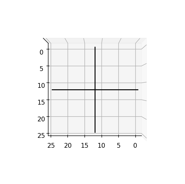
To visualize the geometry of the streamlines, you can display them using
matplotlib.
import matplotlib.pyplot as plt
from mpl_toolkits.mplot3d import Axes3D

fig = plt.figure(figsize=(5, 5), dpi=150)
ax = fig.add_subplot(111, projection='3d')
ax.plot(tractogram[0][:,0], tractogram[0][:,1], tractogram[0][:,2], 'k')
ax.plot(tractogram[1][:,0], tractogram[1][:,1], tractogram[1][:,2], 'k')
ax.view_init(90,90)
ax.set_zticks([])
plt.show()

Building a linear operator
Now that we have a tractogram, we can start using talon.
First, we will voxelize the tractogram by separating each streamline into
voxel elements. If you are familiar with tractography, streamlines are generated
by following peaks of an image. Voxelizing a tractogram is the opposite i.e.
creating peaks from streamlines. In order to voxelize the tractogram, we first
need to provide a list of directions of the possible orientations of the
streamlines represented as an array of unit vectors.
import talon

directions = np.array([[1, 0, 0], [0, 1, 0], [0, 0, 1]], dtype=np.float)
image_shape = (image_size,) * 3
indices, lengths = talon.voxelize(tractogram, directions, image_shape)
Next we define how each streamline direction is projected onto the data.
generators = np.ones((len(directions), 1))
Finally, we build the linear operator \(A\).
A = talon.operator(generators, indices, lengths)
Note that generators can be multidimensional. One way to illustrate this is to use the directions as generators.
G = talon.operator(directions, indices, lengths)
Generating data with a linear operator
To generate data simply multiply (using the @ operator) the linear operator
by a weight vector.
# Using a vector off all ones gives all streamlines equal weight.
x = np.ones(A.shape[1])
b = A @ x

# We can do the same thing with the multidimensional operator.
m = G @ x
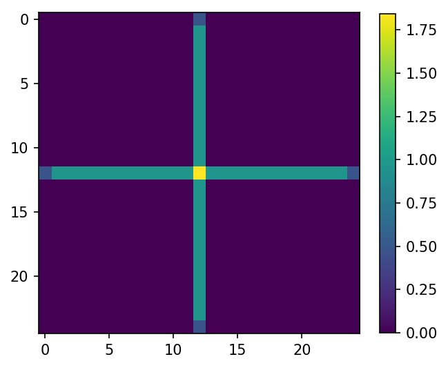
The data vector b can be reshaped into an image and visualized.
image = b.reshape(image_shape)

plt.figure(figsize=(5, 5), dpi=150)
plt.imshow(image[:, :, center])
plt.colorbar(shrink=0.8)
plt.show()
An we obtain the following image which corresponds to the streamline density.
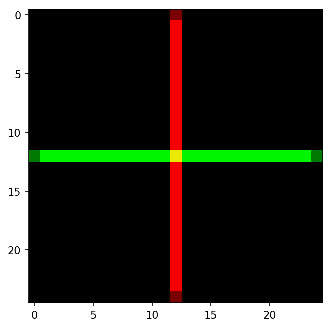
The second data vector can also be visualized, but requires a bit more manipulation.
rgb_image = m.reshape(image_shape + (3,))

plt.figure(figsize=(5, 5), dpi=150)
plt.imshow(rgb_image[:, :, center])
plt.show()
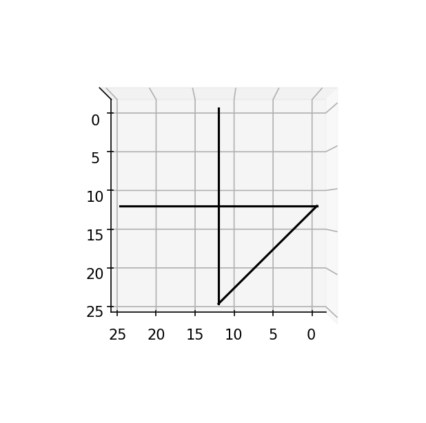
Explaining data with a linear operator
Considering the case where an error in the tractography algorithm generates a spurious streamline in our tractogram. In the case of our example, we simply add a diagonal streamline to tractogram.
diagonal_points = np.array([[0, center, center], [center, image_size - 1, center]])
diagonal_streamline = interp1d([0, 1], diagonal_points, axis=0)(t)

tractogram.append(diagonal_streamline)

# Visualize the new tractogram.
fig = plt.figure(figsize=(5, 5), dpi=150)
ax = fig.add_subplot(111, projection='3d')
ax.plot(tractogram[0][:,0], tractogram[0][:,1], tractogram[0][:,2], 'k')
ax.plot(tractogram[1][:,0], tractogram[1][:,1], tractogram[1][:,2], 'k')
ax.plot(tractogram[2][:,0], tractogram[2][:,1], tractogram[1][:,2], 'k')
ax.view_init(90,90)
ax.set_zticks([])
plt.show()
Given b, the data generated using by the original tractogram, we can use
talon to calculate the contribution of each streamline to the data. In order
to do so, we first have to generate a linear operator using the new
tractogram. In this case, we use also use a set of 1000 equally spaced unit
vectors as directions.
directions = talon.utils.directions(1000)
generators = np.ones((len(directions), 1))
indices, lengths = talon.voxelize(tractogram, directions, image_shape)
Z = talon.operator(generators, indices, lengths)
What we want to find are the streamline contributions x which minimize
In this example it does not make sense to have streamlines with a negative
contribution, therefore, \(\Omega(x)\) will be set as a positivity
constraint. In talon, we can force positivity constraint using the
talon.regularization function.
positivity_constraint = talon.regularization(non_negativity=True)
The resulting regularization term is then given to the talon.solve function
in order to obtain the streamlines contributions.
solution = talon.solve(Z, b, reg_term=positivity_constraint)
print('solution.x = [%.2f, %.2f, %.2f]' % tuple(solution.x))
solution.x = [1.00, 1.00, 0.00]
As it is possible to see, the two original streamlines contribute equally to the data while the third streamline does not contribute.
We can use the talon solution to filter the tractogram and visualize only
the streamlines presenting a non-zero contribution.
# New filtered tractogram.
filtered_tractogram = []

fig = plt.figure(figsize=(5, 5), dpi=150)
ax = fig.add_subplot(111, projection='3d')

for i,s in enumerate(tractogram):

    # If the current streamline contributes to the data.
    if solution.x[i] > 0.0:

        # Add streamline to filtered tractogram.
        filtered_tractogram.append(s)

        # Visualize the streamline.
        ax.plot(s[:,0], s[:,1], s[:,2], 'k')

ax.view_init(90,90)
ax.set_zticks([])
plt.show()